Introduction: The Plan of Action
Hi,
Today we’ll start with a quick recap of what you already know, and on this occasion, we’ll dive a little into theory—but as always, we’ll try to keep it very simple. By the end, you’ll download a free tool to your computer, and we will create a database file. I will show you how to install free, professional tools for working with databases. We will create your first local database file, which in the next lesson will be filled with realistic data from an online store. Get ready for some hands-on practice!
Let’s begin
Reminder
We already know that a DATABASE is a collection of TABLES. You can think of a database as an entire Excel file, and the individual tables as worksheets in that file. Or imagine a cabinet with drawers, where each drawer is a separate table, and in it, precisely organized data.
Let’s look at an example of our table containing customer data:
| id | name | city | phone | date_added | |
| 1 | John Smith | Warsaw | +48251457856 | john.smith234@mail.com | 2025-02-15 14:54 |
| 2 | Jane Doe | Lodz | +48123456789 | jane@janedoe.com | 2023-10-05 10:20 |
Let’s call our table above customers.
It contains an id column – which is the primary key; this value is never repeated within this table. It precisely points to a specific record, or row.
Then we see the columns name, city, phone, email – these are our standard data fields. Finally, we have date_added. In most real systems, such fields, usually named created_at (creation date) or modified_at (last modified date), are standard.
Let’s add a products table to the database
| id | name | supplier | unit | price |
| 1 | Women’s T-shirt XS | 4F | pcs | 75.99 |
| 2 | Sheet Metal (by m2) 😉 | BuildIt | m2 | 150.23 |
| 3 | Jeans | Americanos | pcs | 98.14 |
And again, we have an id field, name, supplier, the unit in which the item is sold (pieces and square meters), and the price per unit.
So, we have two independent tables for now. They are not related in any way. We have a customer index and a product index.
We can display products and customers using SQL.
SELECT * FROM customers; – This will show us all records and all columns from the customers table.
SELECT name, price FROM products WHERE unit = ‘pcs’; – This will display only two columns from the products table for items that are sold in pieces.
Joining Data: The purchases Table and the Power of JOIN!
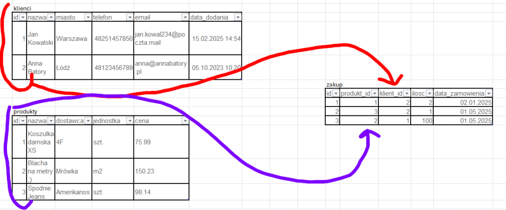
In real e-commerce systems, such independent data is linked together. Imagine a customer buys a specific product in a specific quantity. For this, we need an additional table, which we’ll call purchases:
| id | product_id | customer_id | quantity | order_date |
| 1 | 1 | 2 | 2 | 2025-01-02 |
| 2 | 3 | 2 | 1 | 2025-05-01 |
| 3 | 2 | 1 | 100 | 2025-05-01 |
Before you look further, try to understand what’s happening here by looking at all three tables.
SELECT customers.name, – We select individual columns from three tables using TABLE_NAME.COLUMN_NAME
products.name,
purchases.quantity,
purchases.quantity*products.price AS value, – NOTE!: this is new. We can perform mathematical (and later, statistical) operations on table columns. We name the result using the AS clause as ‘value’
purchases.order_date
FROM purchases – We select the ‘purchases’ table
JOIN customers ON purchases.customer_id=customers.id – We join another table, ‘customers’, and link them by their id fields. Notice, the ‘purchases’ table has ‘customer_id’ and ‘product_id’
JOIN products ON purchases.product_id=products.id – now we add the ‘products’ table
and here is what will happen, we will get this result:
| name | name | quantity | value | order_date |
| Jane Doe | Women’s T-shirt XS | 2 | 151.98 | 2025-01-02 |
| Jane Doe | Jeans | 1 | 98.14 | 2025-05-01 |
| John Smith | Sheet Metal (by m2) 😉 | 100 | 15 023 | 2025-05-01 |
Of course, we see a problem: we have two ‘name’ columns. This is because both tables have columns with the same name, and to fix this, we need to use AS. (e.g., SELECT customers.name AS customer_name, products.name AS product_name).
Local Database!
That’s enough reminding for today. We now have a clear picture of how databases store and link information. Now it’s time to transfer this knowledge to your own computer.
In the previous lesson, I wrote about HeidiSQL (https://www.heidisql.com). It’s a simple application, works well, but it’s only for Windows and Linux. What if you have a Mac OS?
So, a change of plans: I will conduct the course on a free product available for all platforms, including Mac OS: DBeaver Community – https://dbeaver.io/download
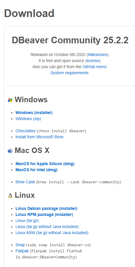
Download the version for your computer. I’m downloading the Windows installer and will base future guides on it.
Installation: Step-by-Step
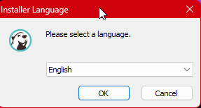
Select your language and click OK, then keep clicking OK and Next until you reach…
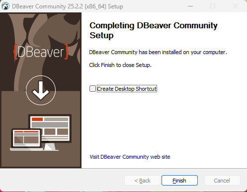
Let’s launch the application.
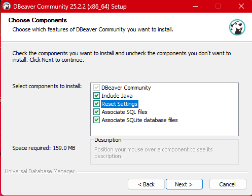
Select all options (unless you use other database software and are a beginner), and then again, click Next and OK until the installation is finished.
DBeaver asks at the very beginning if we want to create a sample database for us! But we won’t do that; we’ll create our own, and in the next lesson, we’ll populate it with data to continue the course.
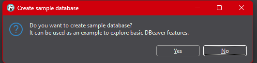
Click No
And we have a view similar to this:
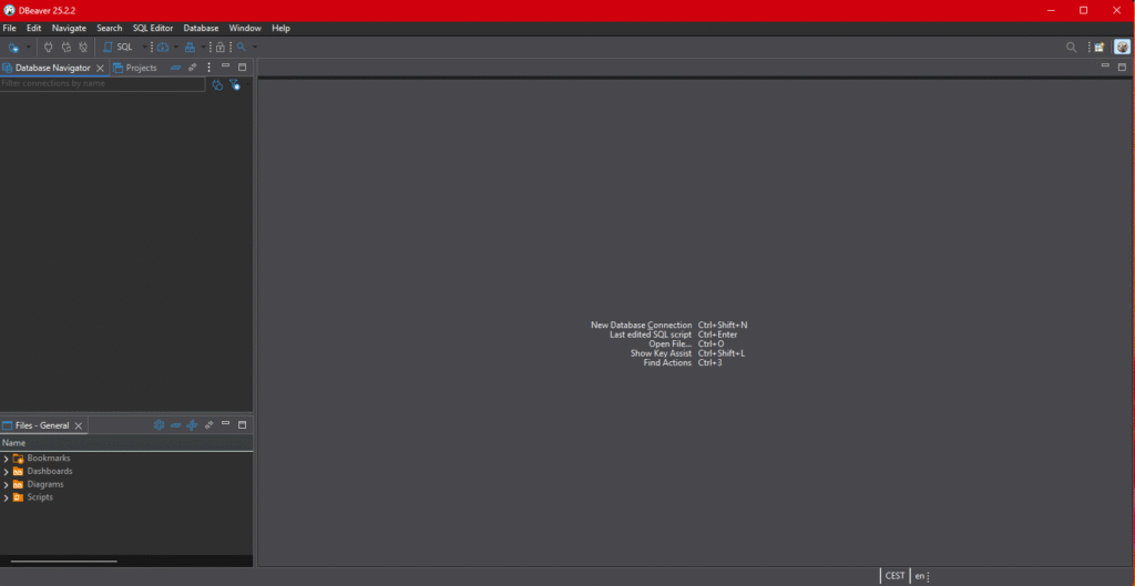
Almost all database tools look practically the same.
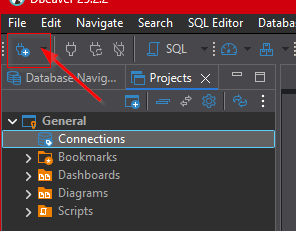
Click the button with the plus icon
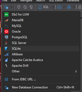
And select SQLite
A window will appear where we click Create
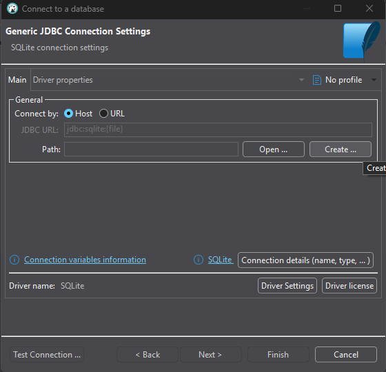
Choose a folder on your computer where our database will be. For simplicity, you can choose the desktop, but I created a folder
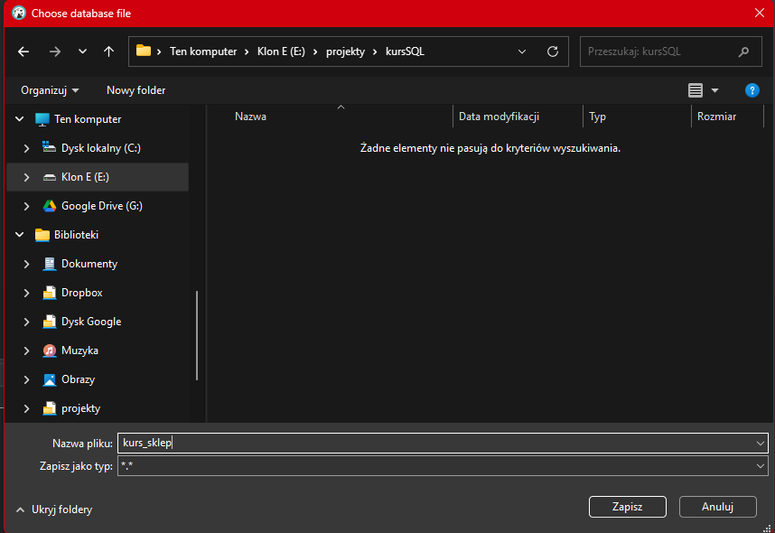
Click Save
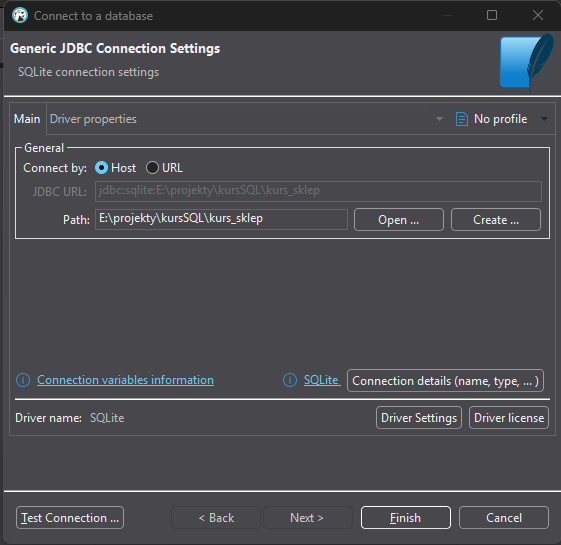
and at the bottom left, select Test Connection
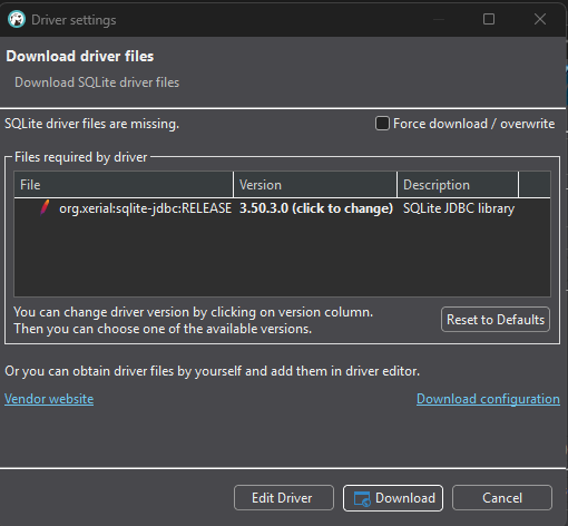
A driver download window will appear; click Download
After that, you’ll get a message that the database is connected
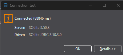
Select OK and then Finish, and you will see the database in the navigator on the left side
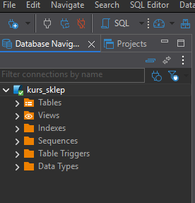
Our database is now waiting for the next lesson, where we will fill it with data and execute our first queries directly on our own computer.
That’s all for today, and I invite you back next week.
0 Comments